• In the past, systematic and discretionary fixed income management have often been seen as antipodes. This may be a false dichotomy that fails to recognize the potential benefits from combining these two orthogonal approaches in a single investment process
• Quantamental fixed income investing is not a wild and distant future dream but is being used by some of the largest managers here and now.
• A case study shows the bits and bobs of how a quantamental fixed income process can be designed in practice. It also reveals the potential risks and benefits of using this investment approach.

———————————-

In my previous article, I made a point about discretionary active managers introducing systematic components to their investment process. This idea raised a few questions, which I thought deserve to be clarified in a separate piece.

This article introduces the concept of quantamental investing. Also known as “active quant”, it is the seamless and disciplined combination of quantitative and discretionary strategies within a single cohesive investment process[1].

Quantamental fixed income investing comes with the promise that “marrying (…) data science and fundamental expertise gives (…) the insights and competitive edge to navigate challenging investment environments” (Klein et. al., 2019, page 11). Only time will tell if this novel approach is worth the hype and can establish itself as a credible and superior solution to traditional discretionary active and/or pure systematic investing. However, just because quantamental investing is still in its early years doesn’t mean it is not worth spending time to study its mechanics and examine its potential benefits. This is where this article comes into play.

The rest of this piece is organized as follows. I start with a brief (and rather personal) introduction of the historically perceived dichotomy between systematic investing and traditional active fixed income management. Following next is a discussion of why combining orthogonal approaches like systematic and discretionary management makes (at least in theory) a lot of sense. Next, I look under the hood of the quantamental fixed income investment process of a large asset manager and compare and contrast its approach with some of my experience and ideas. Finally, I conclude with some high-level thoughts.

Systematic vs discretionary fixed income management

A few years ago, a high-profile quarrel shook the fixed-income investment management industry. I am not talking about a Trash-TV type of fallout, but still a noteworthy spirited exchange between two hugely respected companies from what is otherwise a discreet asset management community.

It all started when AQR Capital Management published two closely related articles[2] investigating the alpha generation skills of active fixed income managers. The second study, cheekily titled “Active Fixed Income Illusions”, looked at a broad range of active fixed income funds across three bond categories – U.S. Agg, Global Agg, and Global Unconstrained Bonds. First, this paper establishes the existence of “impressive active returns across categories over the past two decades” (Brooks et. al., 2020, page 5), broadly confirming previous empirical findings in this area[3]. Next, the study introduces a set of traditional risk premia (duration, corporate credit, emerging markets, and volatility) and uses these to analyze the active returns of a sample of traditional active managers. AQR’s findings – and here is the really controversial part – indicate that “traditional risk premia explain most of the active returns across all (…) [Fixed Income] manager categories” and therefore “active returns of [Fixed Income] managers largely represent a repackaging of traditional risk premia” (Brooks et. al., 2020, page 5). In simple words, AQR claim that traditional active managers fail to produce true alpha; instead, most of their outperformance comes from maintaining long exposure to systematic risk factors, in particular credit beta.

It didn’t take long for traditional active managers to fire back. PIMCO, among them all, published a white paper directly addressing the AQR study. The authors, Baz, Devarajan, Hajo, and Mattu took issue with the AQR’s findings, calling it a “fallacy” to draw conclusions on the nature of alpha based on alpha’s high correlation with a single risk factor (Baz et. al., 2018). To prove this point, Baz et. al. (2018) constructed a hypothetical scenario in which theoretically “true” alpha is constructed (i.e. positive active returns stripped down from any systematic risk factors) which also exhibits a very high correlation with credit beta. Based on these results, the authors conclude that true alpha (even if correlated with systematic credit risk) is valuable, “difficult to source, and one should take it wherever one can find it” (Baz et. al., 2018).

Somehow strangely, this debate feels quite personal to me. The AQR study is co-authored by Scott Richardson. Scott was my Professor at London Business School and taught me all the essentials of systematic fixed income investing. I have nothing but the utmost respect for his work and achievements. Meanwhile, I also sympathize with the other side of the argument because, well, I worked for almost eight years for PIMCO (as those of you who have read my About page know). There is no doubt in my mind that top-skilled discretionary managers can generate true alpha in at least some areas of the fixed income universe.

This is why I believe that pitting systematic against discretionary fixed income management may be a futile discussion, a false dichotomy in a way. Rather than religiously sticking to either systematic or discretionary management, combining the two may be the right way forward. Quantamental investing – i.e., “the disciplined combination of quantitative and fundamental approaches” (Ben Dor et. al., 2021, page 598) could potentially be the solution that offers the best of both worlds. Let’s explore some of the reasons why quantamental investing makes (at least theoretically) so much sense.

Why quantamental investing makes (theoretical) sense

“Diversification is the only free lunch” in investing – a quote attributed to Harry Markowitz and known by pretty much anyone who ever studied portfolio theory. Aiming to improve the overall level of portfolio diversification is hardly a breakthrough goal but, in my view, also the best signpost to guide one’s investment decisions.[4]

Diversification comes in many forms and flavors some of which are pretty obvious. Within a single asset class like fixed income or equities, investors can diversify across regional, country, and industry exposures just to name a few. One level higher, in the context of an entire investment portfolio, diversification can be gained by investing in different asset classes with (hopefully) as little correlation with each other as possible.

There is, however, another dimension that is often overlooked – diversification across styles.  With style diversification, the benefit doesn’t come from adding new asset classes to the portfolio but trading these asset classes in different ways. Trend Following, for example, deploys a systematic approach based on absolute momentum and consisting of long and short trades across bond, equity, and commodity markets. Compare the returns of a Trend Following system with those of a buy-and-hold portfolio of ETFs (covering roughly the same set of markets as the Trend Following strategy) and you will see that the correlation between the two is practically zero.[5]

A similar approach can be implemented within a single asset class like fixed income. Diversifying across styles like, for example, combining discretionary and systematic management techniques, could produce a portfolio with a materially improved risk-adjusted profile vs. any systematic or discretionary portfolio on its own. “Combining active fundamental and quantitative perspectives is also called “orthogonal thinking” – a term used in science to describe a process where unique insights are discovered by drawing on seemingly unrelated perspectives” (Klein et. al., 2019, page 4).  Put more simply, because systematic fixed income strategies exhibit little to no correlation with traditional risk factors[6], combining them with discretionary management approaches within a single quantamental process should yield material benefits in terms of overall portfolio risk-adjusted returns.

Diversifying across orthogonal strategies also means mitigating their inherent weaknesses. Systematic strategies tend to suffer from security selection risk[7] and “have trouble anticipating the complicated human responses of politicians and central bankers that can drive market regime changes” (Klein et. al., 2019, page 4). Meanwhile, discretionary approaches are not foolproof either. Human behavior is plagued with behavioral and cognitive biases which have been extensively studied and well documented.[8] Humans also face capacity constraints when covering an investment universe as vast as the global fixed income markets[9] and therefore struggle to maintain the same amount of analysis precision that machines are capable of[10].

All of this paints a fairly positive (theoretical) picture in favor of quantamental investing. Let’s investigate how this approach can be implemented in practice.

Designing a quantamental investment process

For over 50 years, the active fixed income management industry has worked on the premise that generating alpha invariably requires a skillful combination of top-down and bottom-up investment processes.  This two-dimensional approach pays tribute to the fact that fixed income performance is a combination of global macro risk factors and individual security-specific pricing anomalies.

Historically, both top-down and bottom-up investment decisions have been organized as discretionary processes where human analysis and judgment dictate active portfolio positions. However, with the advancement and availability of more and better data, quantitative/systematic fixed income strategies have arisen as potentially viable supplements to traditional discretionary approaches. As the level of integration between discretionary and systematic increases, the standard two-dimensional fixed income investment process de facto morphs into a four-dimensional quantamental one as Exhibit 1 illustrates.

Exhibit 1: Quantamental investing means transitioning away from a traditional two-dimensional investment process to a four-dimensional one

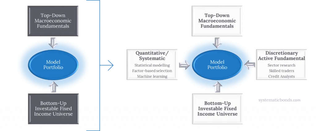
SOURCE: Own illustration adapted from Exhibit 2 in “Quantitative science–active adding to fixed income decisions” by Klein et. al. (2019).

However, the devil is in the details of implementing such a complex four-dimensional concept. Combining “active with quantitative views (…) isn’t to mix them inside a portfolio like a kitchen blender[11]” (Klein et. al., 2019, page 4); it is multi-dimensional problem that requires careful consideration and substantial trade-offs. Let’s investigate how one of the large asset management houses has gone about solving this problem.

A quantamental process in practice

Top-down

This and the following sections are a case study of how combining quantitative/systematic and discretionary investment approaches can be implemented within a single cohesive investment process. It is based on a 2019 paper published by Franklin Templeton and titled “Quantitative science – actively adding to fixed income decisions”.

Franklin Templeton is a large and well-respected asset manager. I have no affiliation with Franklin and am not paid to promote them, their investment process, or any of their products. Any praise of Frankin’s approach is a genuine appreciation of their process. Similarly, any criticism is based on my experience and judgment and has no intention to berate the company or its investment products.

Franklin Templeton’s top-down active quant approach starts with a traditional macroeconomic outlook developed by a team of economists producing forecast ranges for various macroeconomic variables (e.g., inflation, oil prices, exchange rates) (1). These ranges are passed over to Franklin’s data science team and fed into a proprietary algorithm (2). The algorithm produces quantitative views for major fixed income sectors like IG and HY credit, MBS, EM, etc. These quantitative views are, in effect, expected spread distributions with corresponding probability densities, means, and standard deviations (see Exhibit 3 below for an illustration). Next, the quantitative sector views are pitted against the corresponding internal fundamental views, debated among quant and economic team members, and eventually reconciled (3). Next, the reconciled sector views are translated into sector-specific 12M expected returns (4), which in turn get transformed into allocation bands under consideration of volatility, correlations, market regime, and strategy-specific parameters (5).

This whole process is illustrated in Exhibit 2 below.

Exhibit 2: A Top-down active quant process in practice.

SOURCE: “Quantitative science–active adding to fixed income decisions” by Klein et. al., 2019, Exhibit 3. Numeric labels 1-5 have been added by me.

Exhibit 3: Franklin Templeton’s bond spread forecasts (illustrative example)

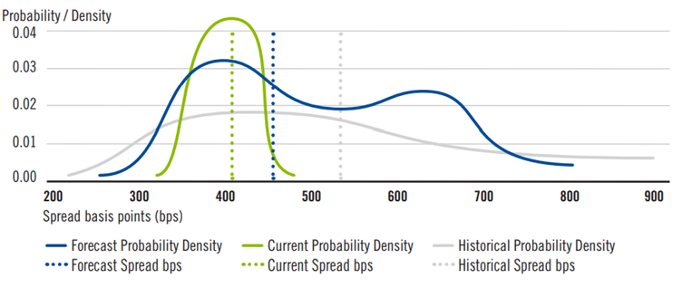
SOURCE: “Quantitative science–active adding to fixed income decisions” by Klein et. al., 2019, Exhibit 4.

Bottom-up

Franklin Templeton’s bottom-up process blends systematic factor investing and fundamental credit research. On the systematic side (1), the company deploys six style factors “spanning value, momentum, and quality categories” (Klein et. al., 2019, page 9). Unlike the more traditional approach of static factor exposures, Franklin Templeton uses proprietary algorithms to dynamically tilt individual factor weights according to the expected credit environment. In parallel, credit research analysts work independently to form their views on individual issuers and industries (2). Next, each side presents their views in “formalized “reconciliation” meetings where credit analysts, portfolio managers, and the data team discuss and debate why and how industry views are either synchronized or opposed” (Klein et. al., 2019, page 8) (3). This process is illustrated in Exhibit 4 below.

Exhibit 4: A Bottom-up active quant process in practice.

SOURCE: “Quantitative science–active adding to fixed income decisions” by Klein et. al., 2019, Exhibit 3. Numeric labels 1-3 have been added by me.

A word about the “Industry/Security Reconciliation” process (labeled #3 in Exhibit 4 above). Its goal is to populate the model portfolio with the highest conviction trades from both quantitative and fundamental perspectives, as illustrated by Exhibit 4 below.

Exhibit 5: Reconciling active fundamental and quant recommendations

SOURCE: “Quantitative science–active adding to fixed income decisions” by Klein et. al., 2019, Exhibit 6.

Critical analysis: Part 1 – some debatable aspects

It is applaudable that Franklin Templeton describe their active quant investment process in such detail, but there is also a limit to what can be learned from a white paper without actually seeing the process from inside. Therefore, if some of the aspects I highlight below misinterpret parts of Franklin’s process, please correct me in the comment section below.

The first thing that catches my eye is Franklin’s extensive use of Machine Learning. Machine Learning (ML) is used in both the top-down process (see label #2 in Exhibit 2 above) and the bottom-up process (see label #1 in Exhibit 4 above). I am somewhat skeptical about the usage of ML because of the low signal-to-noise ratio of financial markets. Also, I prefer the “theory first, data second”-approach (upon which the majority of systematic fixed income strategies are built) which contrasts the “data first”-approach underpinning ML.

Moving away from my personal views, it is interesting to see what the literature has to say about deploying ML in the area of the financial markets. For the sake of brevity, I am not including an overview of the relevant papers here (this can be found in the Appendix). My research paints a fairly nuanced picture in which some studies “demonstrate large economic gains to investors using machine learning forecasts” (Gu et. al., 2019), while other papers point to some of the inherent weaknesses of ML when used in financial markets context. Because the advantages of ML don’t seem to be particularly clear cut, I remain wary of investment processes that rely too much on them.

The second thing worth discussing is the reconciliation discussions between quants and fundamental analysts. Such engagements can be observed in both the top-down (see label #3 in Exhibit 2 above) and the bottom-up process (see label #3 in Exhibit 4 above). I wish Franklin provided a bit more information on how these reconciliation processes are organized in practice. Is it possible for fundamental analysts to completely overwrite opposing quantitative signals? According to Exhibit 4 shown above, the answer is a partial yes. For example, a fundamental “Sell” recommendation always trumps the quantitative signal regardless of its strength (see the orange area labeled “Prioritized Sell” in Exhibit 4). However, for cases that fall under the yellow category “Potential Sells” (see Exhibit 4 above), it is still not entirely clear to me how the reconciliation is done in practice.

The reason I am bringing up the question of the reconciliation process is to voice my conviction that quantitative and discretionary signals should be reconciled in a consistent manner. To clarify, I am not implying that Franklin Templeton is doing this inconsistently. All I am highlighting is that investment managers can reconcile opposing signals by giving preference to either one of them – e.g., fundamental signals are used to overwrite opposing quantitative ones or vice versa. Regardless of which signal is claimed to be more reliable, the key, in my view, is applying this reconciliation approach consistently across the board.

There is also a third reconciliation approach worth mentioning – the integration of fundamental and systematic signals. I first discovered this approach in Robert Carver’s book Systematic Investing[12]. According to it, both the quantitative and fundamental signals are assigned numeric values which are then combined into a single value that ultimately guides the bottom-up positioning of the portfolio. To illustrate, consider issuer A with a quantitative signal of 10 (best = strong overweight) and a fundamental signal of 1 (strong underweight). The combined weighted average signal (assuming equal weights) is 5.5, which would translate into neutral positioning.

Process analysis: Part 2 – the good bits

First, I think it’s important to recognize that Franklin Templeton’s paper is a testament that active quant investing is a genuinely legitimate investment approach capable of managing large pools of AuM. This is essential because there are way too many great strategies that ultimately fail the test of real-world investing due to liquidity, capacity, and other constraints.

Second, looking at the schematic investment process illustrated by Exhibits 2 and 4 above, it becomes clear that quantitative and fundamental approaches can be integrated at virtually every step of the top-down and bottom-up investment processes. What this means is that quantamental investing can be deployed across the full value creation chain and is not confined to a single investment area (e.g., bottom-up security selection only).

Last but not least, it becomes clear that investment managers have a huge level of flexibility when implementing quantamental investing. For example, an investment manager A (let’s call them “fundamental-friendly”) may opt to maintain a completely discretionary top-down approach and sprinkle just a limited amount of quantitative methods onto their otherwise fundamental security selection process. On the other hand, Manager B (let’s call them “quant-excited”) may choose the other extreme – full integration across a fully-fledged quantamental investment process (similar to the case study above), while Manager C (“the moderate one”) may opt for the middle ground. The beauty of quantamental investing, in my view, is that it offers a broad menu of options to suit each investment manager’s unique strengths and preferences.

Conclusion and investment implications

This article introduced the concept of quantamental fixed income investing – an investment approach that potentially offers the combined benefits of discretionary and systematic techniques. Quantamental investing provides investment managers with great flexibility to design unique and distinct investment processes that play into their unique strengths.

We looked at a case study of a large asset manager actively deploying a quantamental fixed income investment process. Based on my industry knowledge, I know there are many more investment houses working in a similar direction.

This prompts me to conclude with a few words to asset owners who may be reading this. I believe asset owners should make a conscious effort to include systematic strategies in their fixed income portfolios (an overview of these can be found here). Asset owners can achieve this either by allocating capital to dedicated systematic products, by selecting investment managers who integrate systematic and discretionary techniques, or by applying some combination of the two. Regardless of the approach, asset owners should continue to carefully monitor their investment managers, measure the overall exposure of their portfolio to alternative systematic risk premia, and actively steer that exposure to a comfortable and reasonable level.

Do please leave a comment in the comment section below or or using the contact form on this website. I would love to hear back from you!

Appendix

Machine Learning in finance: literature overview

In a study from 2019, Gu, Kelly, and Xiu (2019) “demonstrate large economic gains to investors using machine learning forecasts”[13]. The authors trace back these gains to the ability of Machine Learning models to uncover non-linear relationships that are often missed by traditional statistical methods like regression-based techniques. Similarly, Bianchi, Büchner, and Tamoni (2020) “show that machine learning methods (…) provide strong statistical evidence in favor of bond return predictability.” Bianchi et. al (2020) attribute their findings to machine learning models’ ability to capture unspanned macroeconomic information, account for non-linearities, and discriminate between potential explanatory variables when predicting returns for different segments of the fixed income market.

Meanwhile, some work points out the conceptual problems related to ML techniques. An AQR piece[14] highlights four reasons why ML may struggle to produce good results in the context of the financial markets (low signal-to-noise ratio, market evolution, small datasets, need for interpretability). In a study from 2019, Cowgill and Tucker point to the well-known problem of algorithmic bias that ML techniques also tend to suffer from; Athey, 2017 and Athey et al., 2019 highlight how Artificial Intelligence (AI) can infer causal links from statistical correlation and how it handles measurement errors when ML predictions are used for decision making (see e.g. Mullainathan and Obermeyer, 2017; Kleinberg et al., 2018).

Notes

[1] Source: Ben Dor et. al. (2021), page 598

[2] “The Illusion of Fixed Income Diversification” from 2017 and “Active Fixed Income Illusions” from 2020

[3] See e.g., Baz et al. 2017

[4] Of course, there are caveats to this general statement. Increasing the level of diversification comes with the trade-off of higher transaction costs. Sometimes these costs may exceed the benefits from higher diversification. In these cases, more diversification does not lead to higher risk-adjusted returns. For more information on this concept, see Robert Carver’s book “Smart Portfolios”, Part One, Chapter 6 (Carver, 2017, page 141-176).

[5] Based on own calculations. The Trend Following strategy is proxied by a representative portfolio which which trades 55 markets spanning commodities, currencies, interest rates, equities, and volatility. The long-only ETF representative portfolio includes 87 ETFs covering global fixed income, equity, commodities, equity-like alternatives, and bond-like alternatives indices.

[6] See Exhibit 4, Brooks et al. (2018)

[7] See Ben Dor et. al., 2021, page 597

[8] Perhaps the best record of bihavioral and cognitive biases can be found in Daniel Kahneman’s book “Thinking Fast and Slow” (Kahnemann, 2011). Studies have shown that professional investors are not immune to such biases, see e.g., Kudrytsev et. al. (2013), Zahera and Bansal (2018), Jain et. al. (2015), and Shukla et. al. (2020)

[9] See Ben Dor et al., 2021, page 597.

[10] See Klein et. al., 2019, page 4.

[11] You now understand the reason why the tagline photo of this article is a picture of a kitchen blender 😉

[12] What follows is an adaptation of information presented in Chapter 8 (pages 125-133) and Chapter 7 (page 115) from Robert Carver’s 2015 book “Systematic Trading”, (Carver, 2015).

[13] This study is also cited by Franklin Templeton

[14] AQR Learning Center. n.d. Machine Learning: Why Finance is Different. [online] Available at: <https://www.aqr.com/Learning-Center/Machine-Learning/Machine-Learning-Why-Finance-Is-Different> [Accessed 4 March 2022].

References

AQR Alternative Thinking, 2017. The Illusion of Active Fixed Income Diversification. 4Q17.

AQR Learning Center. n.d. Machine Learning: Why Finance is Different. [online] Available at: <https://www.aqr.com/Learning-Center/Machine-Learning/Machine-Learning-Why-Finance-Is-Different> [Accessed 4 March 2022].

Athey, S. and Imbens, G.W., 2019. Machine learning methods that economists should know about. Annual Review of Economics, 11, pp.685-725

Baz, J., Mattu, R., Moore, J., and Guo H., (2017), “Bonds are Different: Active Versus Passive Management in 12 Points.” PIMCO Quantitative Research.

Baz, J., Devarajan, M., Hajo, M., and Mattu, R., (2018), “When Alpha Meets Beta: Managing Unintended Risk in Active Fixed Income.” PIMCO Quantitative Research.

Ben Dor, A., Desclée, A., Dynkin, L., Hyman, J. and Polbennikov, S., 2021. Systematic investing in credit. Hoboken, New Jersey: John Wiley & Sons, Inc.

Bianchi, D., Büchner, M. and Tamoni, A., 2021. Bond risk premiums with machine learning. The Review of Financial Studies, 34(2), pp.1046-1089.

Brooks, J., Palhares, D. and Richardson, S., 2018. Style Investing in Fixed Income. The Journal of Portfolio Management, 44(4), pp.127-139.

Brooks, J., Gould, T. and Richardson, S., 2020. Active Fixed Income Illusions. The Journal of Fixed Income, 29(4), pp.5-19.

Carver, R., 2015. Systematic trading. Hampshire, Great Britain: Harriman House Ltd.

Carver, R., 2017. Smart Portfolios A Practical Guide to Building and Maintaining Intelligent Investment Portfolios. Hampshire, Great Britain: Harriman House Ltd.

Cowgill, B. and Tucker, C., 2017. Algorithmic bias: A counterfactual perspective. NSF Trustworthy Algorithms.

Gu, S., Kelly, B. and Xiu, D., 2019. Empirical Asset Pricing via Machine Learning. Chicago Booth Research Paper, (1818-04).

Jain, R., Jain, P. and Jain, C., 2015. Behavioral biases in the decision making of individual investors. IUP Journal of Management Research, 14(3), p.7.

Kahneman, D., 2013. Thinking, Fast and Slow. New York, United States of America: Farrar, Straus and Giroux.

Kudryavtsev, A., Cohen, G. and Hon-Snir, S., 2013. ‘Rational’or’Intuitive’: Are behavioral biases correlated across stock market investors?. Contemporary economics, 7(2), pp.31-53.

Klein, P., Runkel, T. and Thoutireddy, P., 2019. Quantitative science—actively adding to fixed income decisions. Franklin Templeton Thinks Fixed Income Markets, (October 2019).

Kleinberg, J., Lakkaraju, H., Leskovec, J., Ludwig, J. and Mullainathan, S., 2018. Human decisions and machine predictions. The quarterly journal of economics, 133(1), pp.237-293.

Mullainathan, S. and Obermeyer, Z., 2017. Does machine learning automate moral hazard and error?. American Economic Review, 107(5), pp.476-80.

Shukla, A., Rushdi, D., Jamal, N., Katiyar, D. and Chandra, R., 2020. Impact of behavioral biases on investment decisions ‘a systematic review’. International Journal of Management, 11(4).

Zahera, S.A. and Bansal, R., 2018. Do investors exhibit behavioral biases in investment decision making? A systematic review. Qualitative Research in Financial Markets.

Disclaimer

The information in this article is for personal, non-commercial use only. All content of this article is for general informational purposes only. No information included in this article is investment advice of any kind. Plamen Todorov (“The Provider”) is a publisher and not an investment advisor. The Provider does not make any investment recommendations, nor does the Provider intend to influence users of this article in their personal investment decisions. None of the ideas in this article are meant to be construed as professional and / or financial advice. Readers of this article are solely responsible for their investment decisions. In exchange for using this Website and reading this article, you agree not to hold the Provider or any third party service provider which is connected to this website liable for any possible claim for damages arising from any decision you make based on information or material made available to you through this website.
© 2022 Systematic Bonds. All rights reserved. Plamen Todorov holds the international copyright to all content on this website. Any usage of text or images from this website is permitted only with the prior written consent of Plamen Todorov.